import polars as pl
import polars.selectors as cs
import seaborn as sbn
import matplotlib.pyplot as plt

plt.style.use('ggplot')
plt.rcParams['figure.figsize'] = (15, 5)
print(pl.__version__)

1.6.0

Okay! We’re going back to our bike path dataset here. I live in Montreal, and I was curious about whether we’re more of a commuter city or a biking-for-fun city – do people bike more on weekends, or on weekdays?

4.1 Adding a ‘weekday’ column to our dataframe

First, we need to load up the data. We’ve done this before.

bikes = pl.read_csv('../data/bikes.csv', separator=';', encoding='latin1', try_parse_dates=True)
bikes.plot.line(x='Date', y='Berri 1').properties(width='container')
sbn.lineplot(bikes, x='Date', y='Berri 1')

<Axes: xlabel='Date', ylabel='Berri 1'>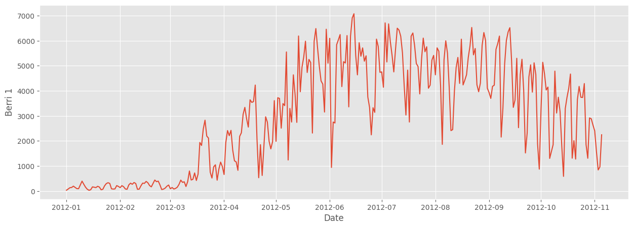

png

Next up, we’re just going to look at the Berri bike path. Berri is a street in Montreal, with a pretty important bike path. I use it mostly on my way to the library now, but I used to take it to work sometimes when I worked in Old Montreal.

So we’re going to create a dataframe with just the Berri bikepath in it

berri_bikes = bikes.select('Date', 'Berri 1')

berri_bikes.head()

shape: (5, 2)

Date	Berri 1
date	i64
2012-01-01	35
2012-01-02	83
2012-01-03	135
2012-01-04	144
2012-01-05	197

Next, we need to add a ‘weekday’ column. Firstly, we can get the weekday from the Date column. It’s basically all the days of the year.

berri_bikes['Date']

shape: (310,)

Date
date
2012-01-01
2012-01-02
2012-01-03
2012-01-04
2012-01-05
…
2012-11-01
2012-11-02
2012-11-03
2012-11-04
2012-11-05

You can see that actually some of the days are missing – only 310 days of the year are actually there. Who knows why.

Polars has a bunch of really great time series functionality, so if we wanted to get the day of the month for each row, we could do it like this:

berri_bikes['Date'].dt.ordinal_day()

shape: (310,)

Date
i16
1
2
3
4
5
…
306
307
308
309
310

We actually want the weekday, though:

berri_bikes['Date'].dt.weekday()

shape: (310,)

Date
i8
7
1
2
3
4
…
4
5
6
7
1

These are the days of the week, where 1 is Monday. I found out that 1 was Monday from the documentation.

Now that we know how to get the weekday, we can add it as a column in our dataframe using the df.with_columns function. This function behaves a lot like df.select except that it also preserves the original columns of the DataFrame (overwriting any re-defined columns).

berri_bikes = berri_bikes.with_columns(
    weekday = pl.col('Date').dt.weekday()
)
berri_bikes.head()

shape: (5, 3)

Date	Berri 1	weekday
date	i64	i8
2012-01-01	35	7
2012-01-02	83	1
2012-01-03	135	2
2012-01-04	144	3
2012-01-05	197	4

4.2 Adding up the cyclists by weekday

This turns out to be really easy!

Dataframes have a .group_by() method that is similar to SQL groupby, if you’re familiar with that. I’m not going to explain more about it right now – if you want to to know more, the documentation is really good.

In this case, berri_bikes.group_by('weekday').agg(sum) means “Group the rows by weekday and then add up all the values with the same weekday”.

weekday_counts = (
    berri_bikes
    .group_by('weekday')
    .agg(pl.col('Berri 1').sum())
    .sort('weekday')
)
weekday_counts

shape: (7, 2)

weekday	Berri 1
i8	i64
1	134298
2	135305
3	152972
4	160131
5	141771
6	101578
7	99310

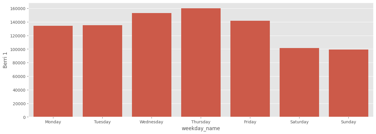
It’s hard to remember what 1, 2, 3, 4, 5, 6, 7 mean, so we can fix it up and graph it:

days_df = pl.DataFrame(
    data={
        "weekday" :range(1, 8),
        "weekday_name": ['Monday', 'Tuesday', 'Wednesday', 'Thursday', 'Friday', 'Saturday', 'Sunday']
    },
    schema_overrides={'weekday':pl.Int8} # Make sure the type matches our weekday_counts dataframe
)
weekday_counts = weekday_counts.join(days_df, on='weekday')
weekday_counts

shape: (7, 3)

weekday	Berri 1	weekday_name
i8	i64	str
1	134298	"Monday"
2	135305	"Tuesday"
3	152972	"Wednesday"
4	160131	"Thursday"
5	141771	"Friday"
6	101578	"Saturday"
7	99310	"Sunday"

sbn.barplot(weekday_counts, x='weekday_name', y='Berri 1')

<Axes: xlabel='weekday_name', ylabel='Berri 1'>

png

So it looks like Montrealers are commuter cyclists – they bike much more during the week. Neat!

4.3 Putting it together

We scan and join the dataframes in lazy mode so data is only computed when requred by the process.

# scan_csv is lazy method that optimizes query only once data is needed to plot.
bikes = pl.scan_csv('../data/bikes.csv', separator=';', encoding='utf8', try_parse_dates=True)

# get weekday data for Berri 1 path
berri_bikes = bikes.select('Berri 1', weekday = pl.col('Date').dt.weekday())

# Add up the number of cyclists by weekday
weekday_counts = (
    berri_bikes.group_by('weekday')
    .agg(pl.col('Berri 1').sum())
    .join(days_df.lazy(), on='weekday')
    .sort('weekday')
)
sbn.barplot(weekday_counts.collect(), x='weekday_name', y='Berri 1')

<Axes: xlabel='weekday_name', ylabel='Berri 1'>

png